E-Beam System Basics 3:
Dose, Machine Grid, and Exposure Grid / Shot Pitch
A critical exposure variable is the e-beam dose, in essence, how many electrons per unit area of exposure. The typical units of e-beam exposure dose are micro-Coulombs per Square Centimeter. (1)
Typical e-beam doses for our resists and 100 kV electrons in our system are in the hundreds of uC/cm^2. The exact dose you need to use for your work will have to be determined experimentally, and for exacting work, you may have to carefully control and modulate the exposure dose between different parts of your pattern. Some of the reasons why the empirical determination is necessary, ie, why I can’t just give you an exact dose to use in all cases include:
- E-Beam Forward Scattering. As the electron beam passes through the layer of resist on your wafer, the beam spreads due to beam/solid interactions.
- E-Beam Back-scattering. When the e-beam hits the substrate layer beneath the resist, some of the electrons will backscatter, across a wide angular distribution. This creates a more diffuse energy distribution both right in the region of the primary exposure, but also has longer-range impacts up to microns away from your pattern. In general, backscattering yield varies with the square of the atomic mass of your substrate layers, so exposing on a heavy element such as a gold film suffers from far more backscattering effects than a lighter material such as silicon.
- Resist Thickness. Optimum dose will vary with resist thickness.
- Resist Processing History. Required dose will also vary with the thermal processing history of your resist. This is far more pronounced for some resists than other resists. Materials classified as “Chemically Amplified Resists” are particularly sensitive the pre-bake and post-bake temperature and time variations.
- Develop Conditions.
- E-Beam Intra-shape Proximity Effect. The geometry-dependent effects the scattering behaviors mentioned above give rise to two classes of “proximity effects”. The intra-shape Proximity Effect causes smaller shapes to be under-exposed relative to larger shapes written with the same dose. You can think of this effect being that each pixel in a smaller shape gets less exposure from scattered electrons, because there are fewer neighboring exposed pixels.
- E-Beam Inter-shape Proximity Effect. Shapes exposed are also effected by other nearby shapes, with electrons scattering through the intervening resist. Densely-packed shapes will strongly interact, providing much “cooperative exposure” between the shapes, and will thus require a lower exposure dose than sparse, isolated shapes, which get fewer scattered electrons and will thus be under-exposed relative to their cousins with closer neighboring shapes.
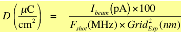
So, how is dose computed? Thinking back to the point-by-point exposure diagram on the previous page, the dose depends on the beam current used for exposure, the dwell time at each pixel, and the spacing of those pixels. This formula is the master formula for dose computation, although you will note that here, I’m not using Dwell Time at each pixel, I’m using the inverse of this, or the “Exposure Frequency” in Pixels per Second. All of the units in this formula are the commonly used units:
Dose is in uC/cm^2
Beam Current is in pA
Exposure Clock Frequency is in MHz (10^6 pixels per second)
Exposure Grid spacing is in nm
(The 100 factor just makes all the units work out. )
Of course, the machine does exactly the same calculation when you enter a beam current, exposure grid and desired resist dose in order to set the exposure frequency.
I've also written some web calculators to do various dose computations for you. All of these are based on the preceding equation:
Compute Area Exposure Dose, given an EOS Mode, Beam Current, Shot Pitch (Exposure Grid, or GridExp), and Exposure Clock (Fshot)
Compute Exposure Clock Rate, given an EOS Mode, Beam Current, Shot Pitch, and Area Exposure Dose,
Compute Minimum Area Exposure Dose possible, given an EOS Mode, Beam Current, and Shot Pitch
Compute Minimum Shot Pitch possible, given an EOS Mode, Beam Current, and Minimum Dose needed
The JBX-6300FS expresses different doses as a Modulation factor times a base dose. The following two calculators translate between dose and MODULAT values, useful when writing Job Files.
Dose From MODULAT, given a Base Dose and MODULAT value, computes actual Dose.
MODULAT from Actual Dose, given a Base Dose and a desired Actual Dose, computes MODULAT value to use.
Exposure Grid vs Machine Grid -- Shot Pitch
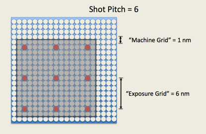
If you’re observant, you might have noticed that earlier, I was talking about “Machine Grid”, and now I’m referring to “Exposure Grid”. Aren’t they the same thing? The answer is “No, usually not.” It turns out that “Machine Grid” spacing, which you might remember for our system is either 1.0 nm in 4th lens mode, or 0.125 nm in 5th lens mode, is a far finer grid than we can meaningfully use in most practical exposures. The limiting factor is a very important system hardware limitation in the factors of the above equation. The hardware of our JBX-6300FS is limited to a maximum “Clock Speed” or “Writing Frequency”, what I’ve labeled “Fshot” above, of 50 MHz. Since resist sensitivity is generally a property of the polymer formulation and can’t really be changed much, the upper limit of “Fshot” of 50 MHz means there are limits imposed on the possible values of beam current and grid size. The system handles this situation by introducing a controllable variable called “Shot Pitch”, which changes the beam stepping pitch, or exposure grid, to be any even integer multiple of the machine grid.
![]()
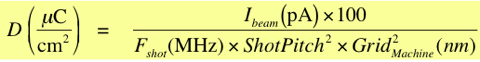
Simple substitution then gives the most basic from of the Exposure Dose Equation:
This contains all of the fundamental variables you’ll have to work with in choosing your exposure conditions.
The Shot Pitch is constrained to being an even multiple of the machine grid size. The figures here illustrate the effects of Shot Pitch 4 and Shot Pitch 6, which in 4th lens equates to an Exposure Grid of 4 nm or 6 nm, while in 5th-lens mode, Shot Pitch 4 gives an exposure grid of 0.5 nm, while for Shot Pitch 6, exposure grid is 0.75 nm. In these figures, only the red pixels will actually be written.

The Shot Pitch is defined in the .JDF file using the SHOT command.
Exposure Doses
The system design allows for up to 256 unique dose values to be exposed in each and every pattern file exposed. This is a significantly powerful feature, because it allows both a great deal of flexibility and control over the minute aspects of the exposure. Specifically, it allows you to compensate, either manually or automatically, for effects due to electron scattering or substrate differences, by assigning different doses to different shapes within your pattern, a process known as Proximity Effect Correction.Within your pattern preparation, each shape is assigned an index value, ranging from 0 (the default) to 255. These index values are called Shot Ranks. All of the shapes on each of the Shot Rank values is exposed with the same dose value, with the actual dose value being assigned in the Job File, not the pattern file. Again, the pattern file contains shapes, each of which is assigned to some index value between 0 and 255, and the actual exposure dose (ie, clock rate) for each of those index values is assigned in the Job File. The relative doses are defined using the JDF MODULAT command in what is called a Shot Modulation Table.
How to choose values for exposure variables?
As I said above, the necessary Exposure Dose depends on the resist and processing conditions, and usually has to be optimized empirically.
The Beam Current Ibeam depends on the system setup. At any time, there are a fixed number of beam currents available for use, as listed in this table. If at any time, you feel you need a different beam current setup, talk with me and I may be able to set up a new current condition file for your needs. There are practical operating limits for beam current, which depend on which final aperture is used, and the resulting beam diameter.
The Exposure Clock Fshot is limited by the system hardware to the upper limit of 50 MHz, or 50 million pixels per second.
The Machine Grid, GridMachine, depends on which lens mode you choose to operate in, 4th lens = 1 nm, 5th lens = 0.125 nm.
And Shot Pitch is constrained to be 1, or an integer multiple of 2, in other words, {1, 2, 4, 6, 8, 10, 12, 14, 16, 18, 20.... }
See the Next Page for information on how to pull this all together into choosing your actual operating conditions.