• EBeam Home
• News
• Remote Work
• Training
• Documentation
  • Overview
  • Safety
  • CAD
  • PatternPrep
    • Getting Started
    • File Names & Dirs
    • File Transfer: EBSEND
    • Fracturing
    • Bias
    • Bordering or Sleeving
    • Field Placement
    • Dose: Manual
    • Dose: Auto via Filter
    • JBXFiler
    • Proximity Correction
    • Beamer Manual
    • Beamer Videos
    • Beamer Release Notes
    • JEOL Appl Note
    • Beamer Versions
  • JobFiles
  • Exposure
  • Alignment
  • JEOL Documentation
  • Operation
• Process
• Reference
• Site Index
• Site Map
• Website Updates

Field Placement

In an ideal ebeam, any shape you write anywhere in the field will be perfect. But, until someone invents that ideal ebeam (and don't hold your breath waiting!), there are some optimizations you can do to avoid some of the imperfections that come with all real ebeams. One detail is the placement of your writing shapes within the ebeam field. Although the system has correction for deflection-induced distortion, defocus and astigmatism, you will still get the best results if you write as much as possible in the center of the ebeam field. This is particular true as feature sizes go smaller.

Simple example, a small pattern

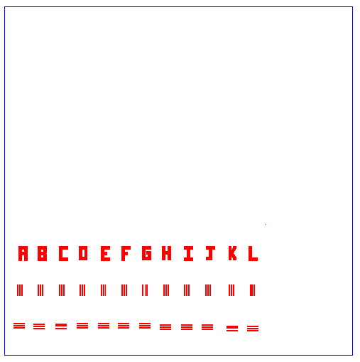
So if, for example, you have just a small pattern, smaller than a field size. If you use LayoutBEAMER to fracture and EXPORT that data to JEOL format, using the default options, that pattern might look like this: The pattern data is drawn in red, the field boundary in blue. My data is all clustered down in the lower left corner.



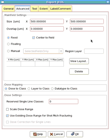
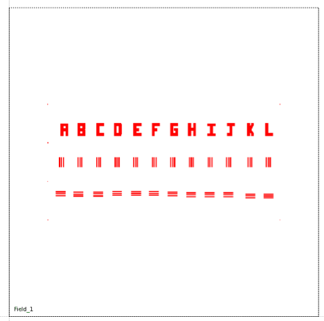
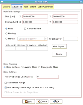
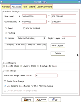
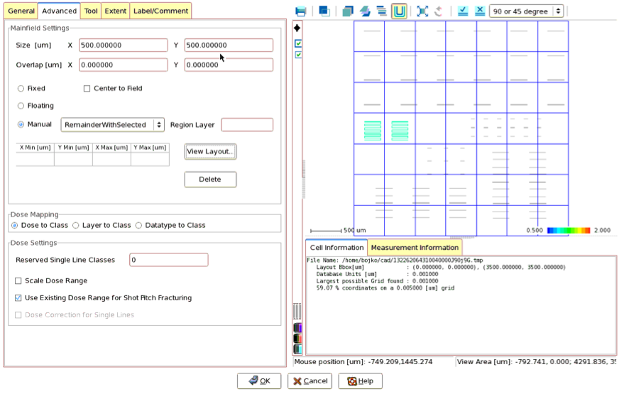
But if I edit the parameters of the JEOL EXPORT box, and look in the Advanced tab, I see some Mainfield Settings. In this example, I just check the "Center to field" checkbox, and after re-fracturing, the output is now:




And, true to its name, the data is now centered in the output ebeam field. This is generally a better case for improved writing and uniformity.

A more complicated example - a larger, multi-field chip

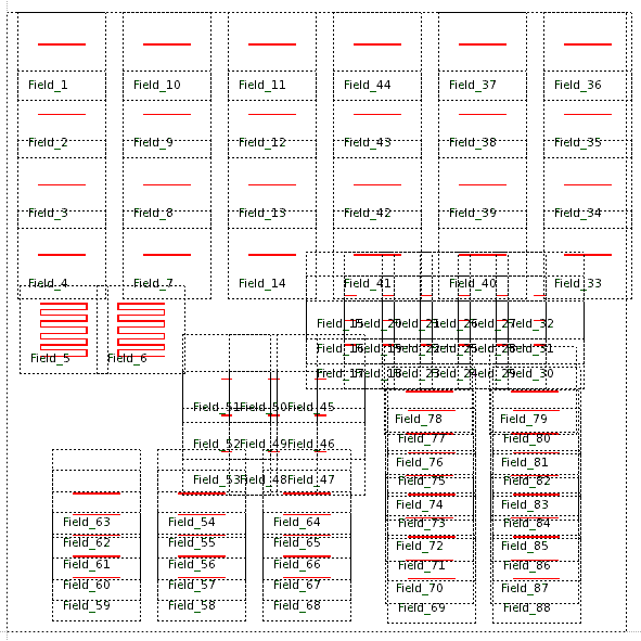
Consider the following prototypical example of a device chip, which one might build if testing transistor materials.


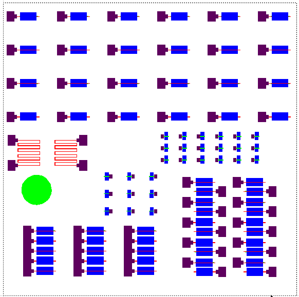
Now, let's view this in LayoutBEAMER, with the default 500 um ebeam fields shown in blue here, and showing on the Gate Metal, often the most critical layer in a typical device.



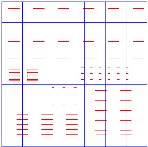
The problem is that some devices are bisected by field stitch boundaries. In this case, the smallest and most critical feature in this device is the gate metal, now shown here in red, with the field boundaries still shown in blue:


This is definitely not optimal, as these gates will have the imperfection of a field stitch right down their middle. What to do? Fortunately, no need to re-design the pattern. Instead, we can work with some features in the EXPORT module, ADVANCED tab to improve the results.

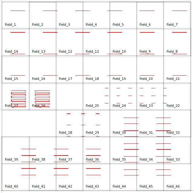
First, let's look at the JEOL output, using the default FIXED field placement option. You can see that LayoutBEAMER has fractured the data just as shown above, but now labeled the output fields in the order they will be exposed. You can also see that empty fields are skipped; no reason to do stage moves with no writing involved.



Now, let's visit the EXPORT JEOL module, ADVANCED tab, and try some options under the Mainfield Settings section. Notice that the default option is "Fixed". This is what you see above -- the fields are placed on a fixed 500 micron field square grid.



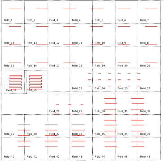
First, let's change this mode from FIXED to FLOATING and re-run the fracture. Here's the output:


"Floating" means that LayoutBEAMER can choose the optimum position for each field, or at least try to. In this case, you see that instead of 46 fields (and thus 46 stage steps) in the Fixed example above, we now have just 27 fields -- this will save considerable time in stage moves, but more importantly, you notice that we have almost entirely eliminated gates being split by field stitch boundaries. The only narrow lines now split are in the meander test structures, now split between Fields 16 and 17. Notice that in some places, LayoutBEAMER chose to overlay fields to avoid stitch boundaries. You see this at Fields 18, 19 and 20. These fields overlap. No fear, any shapes in the overlap are written only once, in the field in which the shape is best written, that is, where the shape is closest to the field center.

This is a big improvement, but still not perfect -- that meander stitched between Field 16 and 17 isn't optimal. LayoutBEAMER tried, but didn't quite get this one perfect.
All hope is not lost, we just have more work to do.

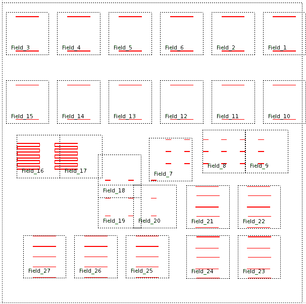
Let's assume we want absolute perfection here. We really don't like the way the gates are written at the field extremes - you can see this especially in Fields 21 - 27 -- they all have gates at both maximum and minimum Y values within the field. This is a worst case for linewidth uniformity. If we want to go for maximum uniformity, we want each gate written at the center of its own field. We're going to use a LayoutBEAMER feature that allows Manual placement of each field, but we'll use a trick to define the manual fields automatically.
First, we add a few steps to the flow. We split the pattern, and use a BIAS module to bias everything UP by 18 microns (you have to determine this best value for this by trial and error), and, this is important, output the biased data to a different layer, set under the TARGET tab of the BIAS module. In this case, I used Layer 40, which was otherwise unused in my Layout.



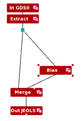
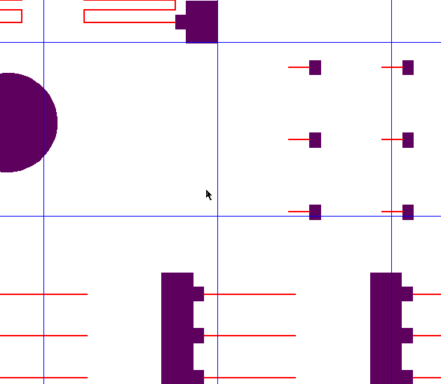
Then we merge the data back together, so I still have my original gates I want to write, plus a new layer, 40, with a large border around each gate. Here's a view of those two layers, at the MERGE module in this flow:


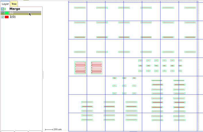
Now, in the EXPORT JEOL module, Advanced tab, this time select Mainfield Settings, MANUAL, Selected Fields Only, and put in Layer 40 as the Region layer (remember Layer 40 is the biased-up layer we just defined above.)



Now, here's what this gives us:


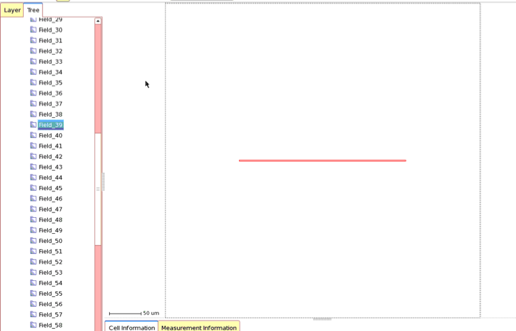
Looks busy, and it is. We now have 88 separate fields, so more stage moves, but, importantly, each gate is now written in the center of its own field. LayoutBEAMER will even allow you to see each field individually, since the aggregate drawing above is a bit hard to decipher. On the left side of the viewer, you can choose Tree, and then expand the drop-down to get a listing menu showing each field. You can then step through these and see each field in sequence to verify the placement, and lack of field stitch boundaries.




Another option, if absolutely perfection isn't necessary, but you have a few critical devices that you don't want stitched and want centered, is partial manual field placement. Go back to a simple IMPORT, EXTRACT, EXPORT JEOL flow, but this time, in the EXPORT JEOL, Advanced tab, select Manual field placement, but now choose Remainder WIth Selected (blank out any Region Layer that might be there -- you're not using another layer to define fields this time. Now click the "View Layout" button, and a mini-view of the layout opens to the right of the dialog. You may have to move around and resize the dialog a bit to get a usable view. You can, of course, click-drag on the view to zoom in, etc, just like in a normal viewer window.




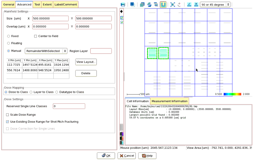
The key here is that we want to manually define a few critical regions. In this case, I want the two meander patterns to be written in their own fields, so I hold down SHIFT, and click-drag a small window over the meaner pattern, which then leaves behind a green-dashed border region, as shown here, plus adds the coordinates of the region to the Manual region table in the left side. Here, I've defined only two regions, but you can define as many as you want, including every shape in the pattern (which would accomplish the same output as the automated example just above.) But let's say the meanders are the only structures that are critical, so we just do those two regions.



Now, when we run the flow, here's the output we get:
The two fields we identified are written centered in their own fields, while everything else is written as default fixed fields.

Summary

The takeaway here is that there is quite a bit of flexibility in field placement, and you can optimize your patterns by taking advantage of these features. There isn't one right answer for your work -- you'll have to look at the needs, what matters most, and maybe even do some trial and error. Discuss this with the ebeam staff if you have questions.